JIT (Just-In-Time) Compilation

Introduction

This document is an extension of Notes 5 and 6 and will focus on how you can help the JIT compiler optimize your code.

We talked before about how Julia runs code as illustrated in the following flowchart:

Julia compiler steps (courtesy of the Julia manual)

JIT Compilation Process

Type inference

Julia uses a complex algorithm to deduce output types from input types. At a high-level, it involves representing the code flow graph as a lattice with some modifications, then running operations on the lattice to determine the types of variables.

SSA (static single-assignment) conversion

SSA form

In SSA, each variable is assigned exactly once. This allows for easier optimization further down the pipeline because the compiler can reason about the flow of data more easily. For example, here is one piece of code before and after SSA:

y = 1
y = 2
x = y

A human can easily see that the first assignment to y is not needed, but it is more complicated for a machine. In SSA form, the code would look like this:

y1 = 1
y2 = 2
x1 = y2

In this form, it is clear that the first assignment to y is not needed, since y1 is never used.

From the manual:

Julia uses a static single assignment intermediate representation (SSA IR) to perform optimization. This IR is different from LLVM IR, and unique to Julia. It allows for Julia specific optimizations.

1. Basic blocks (regions with no control flow) are explicitly annotated.
2. if/else and loops are turned into goto statements.
3. lines with multiple operations are split into multiple lines by introducing variables.

function foo(x)
    y = sin(x)
    if x > 5.0
        y = y + cos(x)
    end
    return exp(2) + y
end;

using InteractiveUtils
@code_typed foo(1.0)

CodeInfo(
1 ─ %1 = invoke Main.sin(x::Float64)::Float64
│   %2 = Base.lt_float(5.0, x)::Bool
└──      goto #3 if not %2
2 ─ %4 = invoke Main.cos(x::Float64)::Float64
└── %5 = Base.add_float(%1, %4)::Float64
3 ┄ %6 = φ (#2 => %5, #1 => %1)::Float64
│   %7 = Base.add_float(7.38905609893065, %6)::Float64
└──      return %7
) => Float64

There are four different categories of IR “nodes” that get generated from the AST, and allow for a Julia-specific SSA-IR data structure.

Optimization passes

The optimization pipeline is a complicated process that involves many steps and can be read about in detail here. The main steps are:

1. Early Simplification
   1. Simplify IR. Branch prediction hints, simplify control flow, dead code elimination, …
2. Early Optimization
   1. Reduce number of instructions. Common subexpression elimination, …
3. Loop Optimization
   1. Canonicalize and simplify loops. Loop fusion, loop unrolling, loop interchange, …
4. Scalar Optimization
   1. More expensive optimization passes. Global value numbering, proving branches never taken, …
5. Vectorization
   1. Vectorize. Earlier passes make this easier and reduce overhead in this step.
6. Intrinsic Lowering
   1. Custom intrinsics. Exception handling, garbage collection, …
7. Cleanup
   1. Last-chance small optimizations. Fused multiply-add, …

Examples

Here are some examples of the techniques the optimization pipeline employs. There are many, many more, but these are some of the common ones as mentioned in the Julia docs:

1. Dead code elimination (DCE): This optimization pass removes code that is never executed.

   1. The conditional block is never executed, so the code inside can be removed:

      function foo(x)
          if false
              x += 1
          end
          return x
      end

2. Constant propagation: This optimization pass replaces variables with their constant values.

   1. The following function can be simplified to return 5:

      function foo(x)
          x = 3
          y = 2
          return x + y
      end

3. Common subexpression elimination (CSE): This optimization pass eliminates redundant computations.

   1. The following function may be compiled to store the value of x^2 in a temporary variable and reuse it:

      function foo(x)
          return x^2 + x^2 + x^2 + x^2
      end

4. Loop unrolling: Loops traditionally have a condition that needs to be checked at every iteration. If the number of iterations is known at compile time, the loop can be unrolled to remove the condition check.

   1. The following loop may be unrolled to remove the condition check:

      a = 0
      for i in 1:4
          a += i
      end

      a = 0
      a += 1
      a += 2
      a += 3
      a += 4

5. Loop fusion: This optimization pass combines multiple loops into one to reduce the number of iterations.

   1. The following two loops may be fused into one:

      a = 0
      b = 0
      for i in 1:4
          a += i
      end
      for j in 1:4
          b += j
      end

      a = 0
      b = 0
      for i in 1:4
          a += i
          b += j
      end

6. Loop interchange: This optimization pass changes the order of nested loops to improve cache performance.

   1. The following nested loops may be interchanged to improve cache performance:

      for i in 1:4
          for j in 1:4
              a[i, j] = i + j
          end
      end

      for j in 1:4
          for i in 1:4
              a[i, j] = i + j
          end
      end

7. Global value numbering (GVN): This optimization pass assigns a unique number to each value computed by the program and replaces the value with its number.

   1. After GVN, the following code can likely be optimized further by CSE (x and z can be replaced with w and y everywhere):

      w = 3
      x = 3
      y = x + 4
      z = w + 4

      w := 3
      x := w
      y := w + 4
      z := y

8. Fused multiply-add (FMA): This optimization combines multiplication and addition instruction into a single instruction if the hardware supports it.

   1. The following code may be compiled to use an FMA instruction:

      mul r1, r2, r3; multiply r2 and r3 and store in r1
      add r4, r1, r5; add r1 and r5 and store in r4

      ; this process is done in a single instruction
      fmadd r4, r2, r3, r5; multiply r2 and r3, add r5, and store in r4

Techniques to help the JIT compiler

We talked last week about some techniques you can use to help the JIT compiler optimize your code, such as putting performance-critical code inside functions, avoiding global variables, typing your variables, and using the const keyword. Here are some more techniques, and you can read about many more in detail here:

There are many good tips recommended by the manual, but here are a few that I think are quite useful or surprising. Most of these boil down to type stability:

Write type-stable code

This code looks innocuous enough, but there is something wrong with it:

pos(x) = x < 0 ? 0 : x;

# This is equivalent to
function pos(x)
    if x < 0
        return 0
    else
        return x
    end
end;

0 is an integer, but x can be any type. This function is not type-stable because the return type depends on the input type. One may use the zero function to make this type-stable:

pos(x) = x < zero(x) ? zero(x) : x;

Similar functions exist for oneunit, typemin, and typemax.

A similar type-stability issue may also arise when using operations that may change the type of a variable such as /:

function foo(n)
    x = 1
    for i = 1:n
        x /= rand()
    end
    return x
end;

The manual outlines several possible fixes:

• Initialize x with x = 1.0
• Declare the type of x explicitly as x::Float64 = 1
• Use an explicit conversion by x = oneunit(Float64)
• Initialize with the first loop iteration, to x = 1 / rand(), then loop for i = 2:10

Be wary of memory allocations

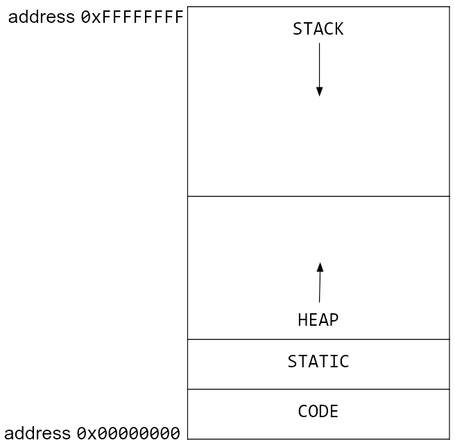
Memory allocation diagram from CS61C

Heap memory allocation can be a bottleneck in your code. If you are allocating memory in a loop, you may be slowing down your code. Here is a toy code segment that repeatedly allocates memory:

function xinc(x)
    return [x, x+1, x+2]
end;

function loopinc()
    y = 0
    for i = 1:10^7
        ret = xinc(i)
        y += ret[2]
    end
    return y
end;

This code, while unrealistic, is a good example of how memory allocation can slow down your code. The xinc function allocates memory every time it is called, and the loopinc function calls xinc several times. This code can be optimized by preallocating memory:

function xinc!(ret, x)
    ret[1] = x
    ret[2] = x+1
    ret[3] = x+2
end;

function loopinc_prealloc()
    y = 0
    ret = [0, 0, 0]
    for i = 1:10^7
        xinc!(ret, i)
        y += ret[2]
    end
    return y
end;

@time loopinc()

  0.405860 seconds (10.00 M allocations: 762.939 MiB, 7.85% gc time)

50000015000000

@time loopinc_prealloc()

  0.003780 seconds (1 allocation: 80 bytes)

50000015000000

Be wary of memory allocations, again

x = rand(1000);
function sum_global()
    s = 0.0
    for i in x
        s += i
    end
    return s
end;
@time sum_global()

  0.010564 seconds (3.68 k allocations: 78.109 KiB, 98.37% compilation time)

493.0660016458528

function sum_local()
    s = 0.0
    x = rand(1000)
    for i in x
        s += i
    end
    return s
end;
@time sum_local()

  0.000018 seconds (1 allocation: 7.938 KiB)

500.14039588612354

The global nature of x prevents the compiler from making many optimizations, especially since it is not typed. Because it is global, and x needs to persist, it requires heap memory allocation. The local version of x is typed and stack-allocated, which allows the compiler to optimize the code better. Stack allocation is usually much faster than heap allocation.

Function barriers

Try to separate functionality into different functions as much as possible. Often there is some setup, work, and cleanup to be done - it is a good idea to separate these into different functions. This will help with compiler optimizations, but it often makes the code more readable and reusable.

Consider the following (strange) code. a will be an array of Int64s or Float64s, depending on the random value, but it can only be determined at runtime. Though this is a contrived example, sometimes there are legitimate cases where things cannot be determined until runtime.

function strange_twos(n)
    a = Vector{rand(Bool) ? Int64 : Float64}(undef, n)
    for i = 1:n
        a[i] = 2
    end
    return a
end;
@time strange_twos(10^6)

  0.058851 seconds (999.54 k allocations: 22.883 MiB, 11.64% gc time, 12.85% compilation time)

1000000-element Vector{Float64}:
 2.0
 2.0
 2.0
 2.0
 2.0
 2.0
 2.0
 2.0
 2.0
 2.0
 ⋮
 2.0
 2.0
 2.0
 2.0
 2.0
 2.0
 2.0
 2.0
 2.0

Instead, separating out the type determination into a different function can help the compiler:

function fill_twos!(a)
    for i = eachindex(a)
        a[i] = 2
    end
end;

function strange_twos_better(n)
    a = Vector{rand(Bool) ? Int64 : Float64}(undef, n)
    fill_twos!(a)
    return a
end;

@time strange_twos_better(10^6)

  0.015667 seconds (1.88 k allocations: 7.752 MiB, 84.70% compilation time)

1000000-element Vector{Int64}:
 2
 2
 2
 2
 2
 2
 2
 2
 2
 2
 ⋮
 2
 2
 2
 2
 2
 2
 2
 2
 2

LoopVectorization.@turbo

Here is some Julia code for a naive matrix multiplication algorithm:

function AmulB!(C, A, B)
    for m ∈ axes(A, 1), n ∈ axes(B, 2)
        Cₘₙ = zero(eltype(C)) # element type
        for k ∈ axes(A, 2)
            Cₘₙ += A[m,k] * B[k,n]
        end
        C[m,n] = Cₘₙ
    end
end;

@time AmulB!(rand(1000,1000), rand(1000,1000), rand(1000,1000))

  1.430879 seconds (6 allocations: 22.888 MiB, 0.61% gc time)

The LoopVectorization.jl package offers the @turbo macro, which optimizes loops using memory-efficient SIMD (vectorized) instructions. However, one can only apply this to loops that meet certain conditions as outlined in the package README.

using LoopVectorization;

function AmulB_turbo!(C, A, B)
    @turbo for m ∈ indices((A,C), 1), n ∈ indices((B,C), 2) # indices((A,C),1) == axes(A,1) == axes(C,1)
        Cₘₙ = zero(eltype(C))
        for k ∈ indices((A,B), (2,1)) # indices((A,B), (2,1)) == axes(A,2) == axes(B,1)
            Cₘₙ += A[m,k] * B[k,n]
        end
        C[m,n] = Cₘₙ
    end
end;

@time AmulB_turbo!(rand(1000,1000), rand(1000,1000), rand(1000,1000))

  0.306820 seconds (6 allocations: 22.888 MiB, 24.73% gc time)

For comparison, here is BLAS matrix multiplication:

using LinearAlgebra;
BLAS.set_num_threads(1);

function BLAS_mul(C, A, B)
    BLAS.gemm!('N', 'N', 1.0, A, B, 0.0, C)
end;

@time BLAS_mul(rand(1000,1000), rand(1000,1000), rand(1000,1000))

  0.053857 seconds (6 allocations: 22.888 MiB)

1000×1000 Matrix{Float64}:
 257.347  250.699  259.414  253.959  …  254.238  244.401  252.12   253.333
 251.841  244.416  256.263  253.47      249.079  247.258  243.135  251.561
 254.138  238.289  254.656  253.811     253.318  252.332  253.364  253.145
 251.22   247.39   256.726  252.656     257.637  244.648  245.677  244.167
 258.11   244.375  257.429  256.45      256.245  246.194  248.168  253.504
 246.412  236.408  246.487  249.249  …  248.086  237.045  238.311  239.815
 262.37   252.564  265.677  260.038     259.599  255.904  260.195  258.454
 255.148  245.884  255.709  255.605     253.4    240.644  248.818  247.677
 256.731  255.629  259.755  257.053     265.486  254.591  252.26   256.328
 253.182  246.763  254.289  252.019     252.003  243.137  243.963  251.144
   ⋮                                 ⋱                             
 254.807  242.887  253.561  253.259     253.612  245.988  252.223  247.241
 247.035  242.627  249.837  249.149     253.356  242.434  244.824  251.413
 248.386  245.498  249.989  251.713     253.862  246.192  251.703  245.239
 252.463  249.915  255.904  250.251     252.322  250.311  250.289  250.606
 249.883  249.381  257.565  256.184  …  254.819  247.749  247.745  248.4
 245.933  239.043  249.694  245.766     246.747  241.968  242.75   245.631
 249.824  246.622  257.6    251.993     253.216  246.655  247.832  247.114
 253.707  248.121  253.528  251.932     254.092  246.517  247.045  251.519
 260.6    255.655  261.687  259.607     263.396  254.516  253.826  256.438